Show the code
library(tidyverse)In B1700 you have started to learn the basics of R. This practical will build on what you have learned already and guide you through the process of cleaning and screening your data using R. You may come across some unfamiliar code during this practical, but with practice, it will become more understandable. We will use the tidyverse package so make sure this is installed and loaded.
library(tidyverse)First we will need to load in our data again. See Practical 1 for more information on how to load your data.
NBADataDF <- as.tibble(read.csv("https://strath-my.sharepoint.com/:x:/g/personal/xanne_janssen_strath_ac_uk/EVSaUwoX8gBCsaNIJ4zz60cB_IbN8fwDkk7gr5BuPdGQng?download=1"))
NBADataDF
# A tibble: 825 × 31
Rk Player.Name Pos Age Tm.Name G GS MP FG FGA FG_Per
<lgl> <chr> <chr> <int> <chr> <int> <int> <dbl> <dbl> <dbl> <dbl>
1 NA Usman Garuba PF 19 HOU 24 2 10 0.8 1.8 0.432
2 NA Josh Giddey SF 19 OKC 54 54 31.5 5.2 12.4 0.419
3 NA Jalen Green SG 19 HOU 67 67 31.9 6.1 14.2 0.426
4 NA Keon Johnson SG 19 TOT 37 12 18.8 2.6 7.4 0.353
5 NA Keon Johnson SG 19 LAC 15 0 9 1.1 3.4 0.333
6 NA Keon Johnson SG 19 POR 22 12 25.5 3.6 10 0.357
7 NA Jonathan Kumi… SF 19 GSW 70 12 16.9 3.4 6.6 0.513
8 NA Moses Moody SG 19 GSW 52 11 11.7 1.5 3.5 0.437
9 NA Daishen Nix SG 19 HOU 24 0 10.9 1.1 2.8 0.403
10 NA Joshua Primo SF 19 SAS 50 16 19.3 2 5.4 0.374
# ℹ 815 more rows
# ℹ 20 more variables: X3P <dbl>, X3PA <dbl>, X3P_Per <chr>, X2P <dbl>,
# X2PA <dbl>, X2P_Per <chr>, eFG_Per <dbl>, FT <dbl>, FTA <dbl>,
# FT_Per <dbl>, ORB <dbl>, DRB <dbl>, TRB <dbl>, AST <dbl>, STL <dbl>,
# BLK <dbl>, TOV <dbl>, PF <dbl>, PTS <dbl>, Player.additional <lgl>Before conducting any analysis, it is crucial to thoroughly screen your data and develop a comprehensive understanding of the variables present in your data set, as well as identify any missing or erroneous data. This initial exploration allows you to ensure the quality and integrity of your data, and aids in making informed decisions throughout the analysis process. To gain an understanding of the variables in our data we often use a data dictionary which for this data set can be found here.
Once you have a thorough understanding of the variables you can start screening. To effectively screen your data, you can perform the following steps:
Examine the structure of your data set: Use functions like str() or summary() to gain an overview of the variables, their types (numeric, character, factor, etc.), and the general structure of the data.
Rename variables: You want to ensure variables names are clear and concise. If they are not you can rename them using colnames()
Investigate missing values: Identify if there are any missing values in your data set and determine how they are represented (e.g., as blank cells, NA, or other placeholders). Utilize functions such as is.na() or complete.cases() to detect missing values and explore their patterns.
Investigate duplicate values: Identify if there are any duplicate values in your data set. Utilize functions such as sort() and unique().
Check for data errors or outliers: Inspect the range and distribution of numerical variables using summary statistics, histograms, or box plots. Look for any extreme or suspicious values that may indicate data errors or outliers.
By thoroughly examining and understanding your data, you can establish a solid foundation for subsequent analysis, ensuring the accuracy and reliability of your findings.
As indicated above, the first step when cleaning data is to examine the structure of your data. By doing so, you can ensure that your variables have been correctly assigned to their respective data types. This step is crucial because it determines the operations and analyses you can perform on your data.
R assigns data into different data types. It is important you understand and know what type has been assigned to each variable. Assigning the wrong data type to a variable can lead to errors or unexpected results. For instance, attempting numerical calculations on a variable that has been mistakenly assigned as a character will lead to an error. Therefore, it is vital to verify the correct assignment of data types. In R you would normally work with 6 different data types:
Numeric - any variable which contains numbers with decimal places (e.g. 2.2, 4.23, 12.3453)
Integer - any variable which contains number without decimal places (e.g. 2, 12, 4)
Character - any variable which contains letters or symbols (e.g. cricket, bat2, 12_12)
Logical - a TRUE or FALSE outcome
Factor - any variable which contains categorical information (e.g. male vs female)
Date - any variable which contains a date
(See Section 5.3 in B1700 for more information)
A convenient and efficient way to gain insights into your data is by utilizing the str() and function. The str() function provides a concise summary of the structure of your data frame, including the data types of each variable.
# Check NBADataDF
str(NBADataDF)
tibble [825 × 31] (S3: tbl_df/tbl/data.frame)
$ Rk : logi [1:825] NA NA NA NA NA NA ...
$ Player.Name : chr [1:825] "Usman Garuba" "Josh Giddey" "Jalen Green" "Keon Johnson" ...
$ Pos : chr [1:825] "PF" "SF" "SG" "SG" ...
$ Age : int [1:825] 19 19 19 19 19 19 19 19 19 19 ...
$ Tm.Name : chr [1:825] "HOU" "OKC" "HOU" "TOT" ...
$ G : int [1:825] 24 54 67 37 15 22 70 52 24 50 ...
$ GS : int [1:825] 2 54 67 12 0 12 12 11 0 16 ...
$ MP : num [1:825] 10 31.5 31.9 18.8 9 25.5 16.9 11.7 10.9 19.3 ...
$ FG : num [1:825] 0.8 5.2 6.1 2.6 1.1 3.6 3.4 1.5 1.1 2 ...
$ FGA : num [1:825] 1.8 12.4 14.2 7.4 3.4 10 6.6 3.5 2.8 5.4 ...
$ FG_Per : num [1:825] 0.432 0.419 0.426 0.353 0.333 0.357 0.513 0.437 0.403 0.374 ...
$ X3P : num [1:825] 0.2 1 2.3 0.9 0.2 1.4 0.7 0.8 0.3 0.8 ...
$ X3PA : num [1:825] 0.8 3.9 6.8 2.7 0.7 4 2.1 2.1 1.1 2.7 ...
$ X3P_Per : chr [1:825] "0.25" "0.263" "0.343" "0.34" ...
$ X2P : num [1:825] 0.6 4.2 3.7 1.7 0.9 2.2 2.7 0.8 0.8 1.2 ...
$ X2PA : num [1:825] 1 8.5 7.4 4.6 2.7 6 4.4 1.4 1.7 2.7 ...
$ X2P_Per : chr [1:825] "0.583" "0.492" "0.502" "0.36" ...
$ eFG_Per : num [1:825] 0.489 0.461 0.508 0.415 0.363 0.428 0.567 0.546 0.455 0.452 ...
$ FT : num [1:825] 0.2 1 2.8 1.1 1.1 1.1 1.9 0.5 0.7 0.9 ...
$ FTA : num [1:825] 0.3 1.5 3.5 1.4 1.4 1.4 2.7 0.7 1.3 1.2 ...
$ FT_Per : num [1:825] 0.714 0.709 0.797 0.804 0.762 0.833 0.684 0.778 0.533 0.746 ...
$ ORB : num [1:825] 0.9 1.8 0.5 0.6 0.4 0.8 0.8 0.3 0.3 0.6 ...
$ DRB : num [1:825] 2.6 6 2.9 1.5 1 1.9 2.6 1.2 1.1 1.6 ...
$ TRB : num [1:825] 3.5 7.8 3.4 2.2 1.4 2.7 3.3 1.5 1.4 2.3 ...
$ AST : num [1:825] 0.7 6.4 2.6 2.1 0.9 2.9 0.9 0.4 1.7 1.6 ...
$ STL : num [1:825] 0.4 0.9 0.7 0.8 0.5 1 0.4 0.1 0.6 0.4 ...
$ BLK : num [1:825] 0.5 0.4 0.3 0.3 0.1 0.5 0.3 0.2 0 0.5 ...
$ TOV : num [1:825] 0.3 3.2 2 1.2 0.5 1.8 1.1 0.3 1.1 1.1 ...
$ PF : num [1:825] 1.2 1.6 1.5 1.9 1.4 2.2 2.1 0.8 0.9 1.6 ...
$ PTS : num [1:825] 2 12.5 17.3 7.2 3.5 9.7 9.3 4.4 3.2 5.8 ...
$ Player.additional: logi [1:825] NA NA NA NA NA NA ...When examining the NBADataDF, it becomes apparent that the X3P_Per and X2P_Per variables are listed as chr (character) type, we would expect this to be num or int. To resolve this issue, we need to investigate why R is categorizing this variable as characters and correct it accordingly.
Typically, R categorizes variables as chr if at least one of the values within the variable contains a character. To address this, we can follow these steps:
Inspect the specific values within these variables that contain characters using the grep() and unique() function. The grep() function enables you to look for patterns within each vector element. The unique() function shows all unique values within a variable.
Evaluate whether the presence of characters is intentional or due to data entry errors. If the characters are indeed part of the data, determine if they can be represented as valid numeric values or if they require special handling.
If the characters are data entry errors, consider cleaning the data by removing or replacing the incorrect characters. This can be done using a function like gsub().
Once the incorrect characters are removed or replaced, convert the variables to the appropriate numerical data type using functions such as as.numeric() or mutate() from the dplyr package.
To inspect which values contain characters, we will first have to tell R which variables we want to inspect.
We will create a vector called VariablesToInspect which contains the following variable names: “3P_Per”, “2P_Per”.
VariablesToInspect <- c("X3P_Per", "X2P_Per")With this variable created we can now create a for loop which uses a combination of grep() and unique() to identify any non-numeric values within our variables.
# Loop through the variables and inspect their unique values

for (var in VariablesToInspect) {
  UniqueValuesDF <- unique(NBADataDF[grep("[a-zA-Z*-]", NBADataDF[[var]]), var])
  cat("Unique values in", var, ":\n")
    print(UniqueValuesDF[[var]])
    cat("\n")
}
Unique values in X3P_Per :
[1] "-"
Unique values in X2P_Per :
[1] "-"rm(UniqueValuesDF)In the code above, a for() loop is used to iterate through each variable name in the VariablesToInspect vector.
The grep("[a-zA-Z*-]", NBADataDF[[var]]) searches for values within the specified variable (NBADataDF[[var]]) that contain lowercase letters (a-z), uppercase letters (A-Z), asterisks (*), or hyphens (-) and returns the row number in which these occur.
The NBADataDF[grep("[a-zA-Z*-]", NBADataDF[[var]]), var] then subsets the NBADataDF dataset based on the values that contain characters in the specified variable.
Adding the unique() function to the code then extracts the unique values from the subset created in the previous step.
Last we want to see the output so cat("Unique values in", var, ":\n") prints a message indicating the variable name being inspected and print(UniqueValuesDF[[var]]) displays the unique values found within the variable. cat("\n") adds a blank line for better readability between variables.
From the output above (and the previous output) we can see that all the inspected variables contain a dash (“-”), which seems to represents missing data. To properly handle these missing values and assign numerical data types to these variables, we need to replace the dashes with NA.
To remove characters, such as the dash, from a variable, we can use the gsub() function in R.
for (var in VariablesToInspect) {
  NBADataDF[[var]] <- gsub("[-]", "", NBADataDF[[var]])
}
rm(VariablesToInspect, var)
After we have removed the characters we can change the data to numerical using mutate() and across() functions. Mutate() allows you to create new columns or in our case modify existing ones. Embedding across within mutate() enables us to change multiple columns at ones.
NBADataDF <- NBADataDF %>%
  mutate(across(c(14,17), as.numeric))
NBADataDF
# A tibble: 825 × 31
Rk Player.Name Pos Age Tm.Name G GS MP FG FGA FG_Per
<lgl> <chr> <chr> <int> <chr> <int> <int> <dbl> <dbl> <dbl> <dbl>
1 NA Usman Garuba PF 19 HOU 24 2 10 0.8 1.8 0.432
2 NA Josh Giddey SF 19 OKC 54 54 31.5 5.2 12.4 0.419
3 NA Jalen Green SG 19 HOU 67 67 31.9 6.1 14.2 0.426
4 NA Keon Johnson SG 19 TOT 37 12 18.8 2.6 7.4 0.353
5 NA Keon Johnson SG 19 LAC 15 0 9 1.1 3.4 0.333
6 NA Keon Johnson SG 19 POR 22 12 25.5 3.6 10 0.357
7 NA Jonathan Kumi… SF 19 GSW 70 12 16.9 3.4 6.6 0.513
8 NA Moses Moody SG 19 GSW 52 11 11.7 1.5 3.5 0.437
9 NA Daishen Nix SG 19 HOU 24 0 10.9 1.1 2.8 0.403
10 NA Joshua Primo SF 19 SAS 50 16 19.3 2 5.4 0.374
# ℹ 815 more rows
# ℹ 20 more variables: X3P <dbl>, X3PA <dbl>, X3P_Per <dbl>, X2P <dbl>,
# X2PA <dbl>, X2P_Per <dbl>, eFG_Per <dbl>, FT <dbl>, FTA <dbl>,
# FT_Per <dbl>, ORB <dbl>, DRB <dbl>, TRB <dbl>, AST <dbl>, STL <dbl>,
# BLK <dbl>, TOV <dbl>, PF <dbl>, PTS <dbl>, Player.additional <lgl>The code above changes all variables at ones. If we only had one variable to change we could have entered
`NBADataDF$X3P_Per <- as.numeric(NBADataDF$X3P_Per)`or simply
`NBADataDF[[14]] <- as.numeric(NBADataDF[[14]])`Upon further inspection there is a few more changes we want to make. Their are a substantial number of variables R treats as characters but are actually Factors (i.e. categorical). Examples are the Pos, Tm.Name variables. We should therefore change these variables from character to factor. We will change these two variables to factors.
NBADataDF<- NBADataDF %>%
  mutate(across(c("Pos", "Tm.Name"), as.factor))
NBADataDF
# A tibble: 825 × 31
Rk Player.Name Pos Age Tm.Name G GS MP FG FGA FG_Per
<lgl> <chr> <fct> <int> <fct> <int> <int> <dbl> <dbl> <dbl> <dbl>
1 NA Usman Garuba PF 19 HOU 24 2 10 0.8 1.8 0.432
2 NA Josh Giddey SF 19 OKC 54 54 31.5 5.2 12.4 0.419
3 NA Jalen Green SG 19 HOU 67 67 31.9 6.1 14.2 0.426
4 NA Keon Johnson SG 19 TOT 37 12 18.8 2.6 7.4 0.353
5 NA Keon Johnson SG 19 LAC 15 0 9 1.1 3.4 0.333
6 NA Keon Johnson SG 19 POR 22 12 25.5 3.6 10 0.357
7 NA Jonathan Kumi… SF 19 GSW 70 12 16.9 3.4 6.6 0.513
8 NA Moses Moody SG 19 GSW 52 11 11.7 1.5 3.5 0.437
9 NA Daishen Nix SG 19 HOU 24 0 10.9 1.1 2.8 0.403
10 NA Joshua Primo SF 19 SAS 50 16 19.3 2 5.4 0.374
# ℹ 815 more rows
# ℹ 20 more variables: X3P <dbl>, X3PA <dbl>, X3P_Per <dbl>, X2P <dbl>,
# X2PA <dbl>, X2P_Per <dbl>, eFG_Per <dbl>, FT <dbl>, FTA <dbl>,
# FT_Per <dbl>, ORB <dbl>, DRB <dbl>, TRB <dbl>, AST <dbl>, STL <dbl>,
# BLK <dbl>, TOV <dbl>, PF <dbl>, PTS <dbl>, Player.additional <lgl>NBADataDF2<-NBADataDFIf we have not already inspected our variable names we can do that using the colnames() function.
colnames(NBADataDF) [1] "Rk" "Player.Name" "Pos"
[4] "Age" "Tm.Name" "G"
[7] "GS" "MP" "FG"
[10] "FGA" "FG_Per" "X3P"
[13] "X3PA" "X3P_Per" "X2P"
[16] "X2PA" "X2P_Per" "eFG_Per"
[19] "FT" "FTA" "FT_Per"
[22] "ORB" "DRB" "TRB"
[25] "AST" "STL" "BLK"
[28] "TOV" "PF" "PTS"
[31] "Player.additional"In the example above we can see that a Player and Tm have a .Name at the end. We may decide this is unnecessary and remove it to shorten the variable name. We can rename variables using rename().
NBADataDF <- NBADataDF %>%
  rename("Player"="Player.Name",
         "Team"="Tm.Name")
As we are replacing a consistent suffix we could also use sub() and gsub() function. So an alternative shorter and more efficient code could be:
for (col in 1:ncol(NBADataDF2)){
  colnames(NBADataDF2)[col]<-sub(".Name", "",colnames(NBADataDF2)[col])
}
rm(col)The example above uses a copy of NBADataDF called NBADataDF2 as the names have already been changed in NBADataDF, so code would not work on that dataset.
The is.na() function helps you identify missing data.
Empty <- is.na(NBADataDF)
head(Empty)
Rk Player Pos Age Team G GS MP FG FGA FG_Per X3P
[1,] TRUE FALSE FALSE FALSE FALSE FALSE FALSE FALSE FALSE FALSE FALSE FALSE
[2,] TRUE FALSE FALSE FALSE FALSE FALSE FALSE FALSE FALSE FALSE FALSE FALSE
[3,] TRUE FALSE FALSE FALSE FALSE FALSE FALSE FALSE FALSE FALSE FALSE FALSE
[4,] TRUE FALSE FALSE FALSE FALSE FALSE FALSE FALSE FALSE FALSE FALSE FALSE
[5,] TRUE FALSE FALSE FALSE FALSE FALSE FALSE FALSE FALSE FALSE FALSE FALSE
[6,] TRUE FALSE FALSE FALSE FALSE FALSE FALSE FALSE FALSE FALSE FALSE FALSE
X3PA X3P_Per X2P X2PA X2P_Per eFG_Per FT FTA FT_Per ORB DRB
[1,] FALSE FALSE FALSE FALSE FALSE FALSE FALSE FALSE FALSE FALSE FALSE
[2,] FALSE FALSE FALSE FALSE FALSE FALSE FALSE FALSE FALSE FALSE FALSE
[3,] FALSE FALSE FALSE FALSE FALSE FALSE FALSE FALSE FALSE FALSE FALSE
[4,] FALSE FALSE FALSE FALSE FALSE FALSE FALSE FALSE FALSE FALSE FALSE
[5,] FALSE FALSE FALSE FALSE FALSE FALSE FALSE FALSE FALSE FALSE FALSE
[6,] FALSE FALSE FALSE FALSE FALSE FALSE FALSE FALSE FALSE FALSE FALSE
TRB AST STL BLK TOV PF PTS Player.additional
[1,] FALSE FALSE FALSE FALSE FALSE FALSE FALSE TRUE
[2,] FALSE FALSE FALSE FALSE FALSE FALSE FALSE TRUE
[3,] FALSE FALSE FALSE FALSE FALSE FALSE FALSE TRUE
[4,] FALSE FALSE FALSE FALSE FALSE FALSE FALSE TRUE
[5,] FALSE FALSE FALSE FALSE FALSE FALSE FALSE TRUE
[6,] FALSE FALSE FALSE FALSE FALSE FALSE FALSE TRUErm(Empty)As you can see from the above, this function shows us if data is missing by giving the cell a TRUE value. However, when working with big datasets this is not very useful. We would normally use the is.na() function within a section of code.
For example, to determine if there are any variables in your data that have no data at all and can potentially be removed, you can compare the total number of cells with no data to the total number of rows in the table. The following code demonstrates how to perform this check:
#screen for empty variables
cat("Test for empty columns","\n","\n")
Test for empty columns
EmptyVar <- which(colSums(is.na(NBADataDF)) == nrow(NBADataDF))
print(EmptyVar)
Rk Player.additional
1 31 The code above sums all the empty cells for each column and compares that to the number of rows in the dataset. It then uses the which() function to tell us for which columns the sum of empty rows and the total number of rows is equal. From the two outputs above, we can observe that there are 2 variables with entirely missing data. We will remove these variables as they won’t be of any use to us.
x=0
for (item in EmptyVar) {
  item <- item-x
  NBADataDF <- NBADataDF[-item]
  x<- x+1
}
rm(EmptyVar, item, x)An alternative option to the code would be: NBADataDF <- NBADataDF[c(-1,-31)]. The first option is more efficient and does not require you to change anything if your data or column numbers would change.
Next we will check if NBADataDF has any missing row data and print the total number of missing data points as well as the missing data per variable.
cat("Total missing data:","\n", sum(is.na(NBADataDF)|NBADataDF==""),"\n")Total missing data:
256 cat("\n","Missing data per variable:","\n")
Missing data per variable: print(colSums(is.na(NBADataDF)|NBADataDF=="")) Player Pos Age Team G GS MP FG FGA FG_Per
0 1 1 1 1 1 1 1 1 16
X3P X3PA X3P_Per X2P X2PA X2P_Per eFG_Per FT FTA FT_Per
1 1 74 1 1 29 16 1 1 98
ORB DRB TRB AST STL BLK TOV PF PTS
1 1 1 1 1 1 1 1 1 We can see from the table that a number of variables have missing values. It is not unusual for data sets to have missing data and sometimes it will just be one missing data point for one athlete, sometimes, variables relate to an event type and therefore will remain empty if the row does not reflect a certain event. However, in some instances the rows are completely empty (i.e. no data is entered for that athlete or event). If that is the case we would like to remove that row. You can do this with the code below:
NBADataDF<-NBADataDF[rowSums(is.na(NBADataDF)) != ncol(NBADataDF), ] The code above compares the total number of empty cells in a row (i.e. rowSums(is.na(NBADataDF))) to the total number of columns (i.e. ncol(NBADataDF). If the total number of missing cells is not equal (i.e. !=) to the total number of columns we will keep the data, otherwise the row will be removed.
If you have paid attention you will have seen no rows have been deleted. The reason for this is that every row has an id, index, period, etc assigned to it. If we know there are rows which may be completely empty or don’t contain any information relevant to us we can still get rid of them by specifying which columns R should check for missing values. In our case, we want only rows which have a player and position assigned to them so we can get rid of those with missing data in that variable.
NBADataDF <- NBADataDF %>%
  filter(Player!="" & Pos!="")
The code above will use filter() to filter the dataset and only include those rows that have no missing data !="" (i.e. not equivalent to ““), in the variables specified. Note how the & (AND) symbol is used to specify that if a row has data in both of these variables the row should be kept. If you only require data in one of these variables you could have used the | (OR) sign.
We have removed some missing data (NBADataDF now contains 824 observations) but there is still a fair few variables with missing data. This is something you may want to look into further. As indicated above, it could be genuine missing data (i.e. the outcome is not relevant to that player) or missing data could be due to inconsistent data collection procedures, data entry errors, or specific conditions under which the data was not recorded (more likely in our case).
For this and future practicals using this dataset we will apply Pairwise Deletion (i.e. analyzing all cases where the variables of interest are present and ignoring missing values), there are however multiple ways to deal with missing variables is discussed in Week 4 of B1700.
Duplicate values in a data set can impact the accuracy and integrity of data analysis. To identify and handle duplicates, you can utilize various functions and techniques. First we would like to sort the data and visually screen it.
#sort data on player, date and innings number
#| code-fold: true
#| code-summary: "Show the code"
NBADataDF <- with(NBADataDF, NBADataDF[order(Player, decreasing=FALSE), ])
head(NBADataDF)
# A tibble: 6 × 29
Player Pos Age Team G GS MP FG FGA FG_Per X3P X3PA
<chr> <fct> <int> <fct> <int> <int> <dbl> <dbl> <dbl> <dbl> <dbl> <dbl>
1 Aaron Gord… PF 26 DEN 75 75 31.7 5.8 11.1 0.52 1.2 3.5
2 Aaron Henry SF 22 PHI 6 0 2.8 0.2 0.8 0.2 0 0.2
3 Aaron Holi… PG 25 TOT 63 15 16.2 2.4 5.4 0.447 0.6 1.6
4 Aaron Holi… PG 25 WAS 41 14 16.2 2.4 5.2 0.467 0.6 1.6
5 Aaron Holi… PG 25 PHO 22 1 16.3 2.3 5.6 0.411 0.7 1.6
6 Aaron Nesm… SF 22 BOS 52 3 11 1.4 3.5 0.396 0.6 2.2
# ℹ 17 more variables: X3P_Per <dbl>, X2P <dbl>, X2PA <dbl>, X2P_Per <dbl>,
# eFG_Per <dbl>, FT <dbl>, FTA <dbl>, FT_Per <dbl>, ORB <dbl>, DRB <dbl>,
# TRB <dbl>, AST <dbl>, STL <dbl>, BLK <dbl>, TOV <dbl>, PF <dbl>, PTS <dbl>In the code, NBADataDF is sorted based on the specified column (i.e., Player) using the order() function. This helps identify duplicate entries that have the same values across these columns. The with() function in R allows you to perform operations on a data frame without having to repeatedly specify the data frame’s name. It temporarily attaches the data frame so you can directly reference its columns without explicitly stating the data frame name each time.
By screening the data visually we do not seem to see any duplicates. However, it is worth doing a more thorough check, especially when working with large datasets like this. To check we can use duplicated() and which() function together. We will ask R which rows are duplicated based on column Player and Team.
# Identify duplicates
which(duplicated(NBADataDF[ ,c("Player", "Team")]))
[1] 7 86 149 217 299 319 369 406 497 599 661 688 818We can now see there are 13 rows with duplicates. To remove duplicates we will again use duplicated().
# Remove duplicates
NBADataDF <- NBADataDF[!duplicated(NBADataDF[ ,c("Player","Team")]), ]
print(NBADataDF)
# A tibble: 811 × 29
Player Pos Age Team G GS MP FG FGA FG_Per X3P X3PA
<chr> <fct> <int> <fct> <int> <int> <dbl> <dbl> <dbl> <dbl> <dbl> <dbl>
1 Aaron Gor… PF 26 DEN 75 75 31.7 5.8 11.1 0.52 1.2 3.5
2 Aaron Hen… SF 22 PHI 6 0 2.8 0.2 0.8 0.2 0 0.2
3 Aaron Hol… PG 25 TOT 63 15 16.2 2.4 5.4 0.447 0.6 1.6
4 Aaron Hol… PG 25 WAS 41 14 16.2 2.4 5.2 0.467 0.6 1.6
5 Aaron Hol… PG 25 PHO 22 1 16.3 2.3 5.6 0.411 0.7 1.6
6 Aaron Nes… SF 22 BOS 52 3 11 1.4 3.5 0.396 0.6 2.2
7 Aaron Wig… SG 23 OKC 50 35 24.2 3.1 6.7 0.463 0.8 2.8
8 Abdel Nad… SF 28 PHO 14 0 10.4 0.9 2.5 0.343 0.3 1
9 Ade Murkey SG 24 SAC 1 0 1 0 0 NA 0 0
10 Admiral S… SF 24 ORL 38 1 12.3 1.4 3.4 0.419 0.7 2.1
# ℹ 801 more rows
# ℹ 17 more variables: X3P_Per <dbl>, X2P <dbl>, X2PA <dbl>, X2P_Per <dbl>,
# eFG_Per <dbl>, FT <dbl>, FTA <dbl>, FT_Per <dbl>, ORB <dbl>, DRB <dbl>,
# TRB <dbl>, AST <dbl>, STL <dbl>, BLK <dbl>, TOV <dbl>, PF <dbl>, PTS <dbl>Now all our variables have been assigned to correct variable type, renamed, and cleaned we can check the actual data itself for errors and outliers. We want to check outliers in numerical variables so we will start by identifying which variables are numerical:
# Create numerical variables data frame
NumericVarsDF <- NBADataDF %>%
  select_if(is.numeric)
NumericVarsDF <-as.tibble(NumericVarsDF)
NumericVarsDF
# A tibble: 811 × 26
Age G GS MP FG FGA FG_Per X3P X3PA X3P_Per X2P X2PA
<int> <int> <int> <dbl> <dbl> <dbl> <dbl> <dbl> <dbl> <dbl> <dbl> <dbl>
1 26 75 75 31.7 5.8 11.1 0.52 1.2 3.5 0.335 4.6 7.7
2 22 6 0 2.8 0.2 0.8 0.2 0 0.2 0 0.2 0.7
3 25 63 15 16.2 2.4 5.4 0.447 0.6 1.6 0.379 1.8 3.7
4 25 41 14 16.2 2.4 5.2 0.467 0.6 1.6 0.343 1.9 3.6
5 25 22 1 16.3 2.3 5.6 0.411 0.7 1.6 0.444 1.6 4
6 22 52 3 11 1.4 3.5 0.396 0.6 2.2 0.27 0.8 1.3
7 23 50 35 24.2 3.1 6.7 0.463 0.8 2.8 0.304 2.3 4
8 28 14 0 10.4 0.9 2.5 0.343 0.3 1 0.286 0.6 1.5
9 24 1 0 1 0 0 NA 0 0 NA 0 0
10 24 38 1 12.3 1.4 3.4 0.419 0.7 2.1 0.329 0.7 1.3
# ℹ 801 more rows
# ℹ 14 more variables: X2P_Per <dbl>, eFG_Per <dbl>, FT <dbl>, FTA <dbl>,
# FT_Per <dbl>, ORB <dbl>, DRB <dbl>, TRB <dbl>, AST <dbl>, STL <dbl>,
# BLK <dbl>, TOV <dbl>, PF <dbl>, PTS <dbl>We now have a dataframe with our 26 numerical variables. Next we can create a loop which will create some summary statistics for us which will help with understanding the data in front of us and identifying any outliers or errors.
# Loop through each numeric variable

for (var in names(NumericVarsDF)) {
  # Calculate summary statistics
  VarSummary <- summary(NumericVarsDF[[var]],na.rm=TRUE)

  # Print summary statistics and outliers
  cat("Variable:", var, "\n")
  print(VarSummary)
  cat("\n")
}
Variable: Age
Min. 1st Qu. Median Mean 3rd Qu. Max.
19.00 23.00 25.00 26.06 29.00 41.00
Variable: G
Min. 1st Qu. Median Mean 3rd Qu. Max.
1.00 12.00 36.00 36.67 61.00 82.00
Variable: GS
Min. 1st Qu. Median Mean 3rd Qu. Max.
0.00 0.00 4.00 16.61 25.00 82.00
Variable: MP
Min. 1st Qu. Median Mean 3rd Qu. Max.
1.00 10.50 17.50 18.25 25.70 43.50
Variable: FG
Min. 1st Qu. Median Mean 3rd Qu. Max.
0.000 1.200 2.400 2.867 3.900 11.400
Variable: FGA
Min. 1st Qu. Median Mean 3rd Qu. Max.
0.000 3.000 5.100 6.377 8.700 21.800
Variable: FG_Per
Min. 1st Qu. Median Mean 3rd Qu. Max. NA's
0.0000 0.3850 0.4410 0.4343 0.5000 1.0000 15
Variable: X3P
Min. 1st Qu. Median Mean 3rd Qu. Max.
0.0000 0.2000 0.7000 0.8699 1.3500 4.5000
Variable: X3PA
Min. 1st Qu. Median Mean 3rd Qu. Max.
0.000 0.800 2.000 2.556 3.900 11.700
Variable: X3P_Per
Min. 1st Qu. Median Mean 3rd Qu. Max. NA's
0.0000 0.2585 0.3310 0.3034 0.3765 1.0000 72
Variable: X2P
Min. 1st Qu. Median Mean 3rd Qu. Max.
0.000 0.700 1.500 1.998 2.800 9.500
Variable: X2PA
Min. 1st Qu. Median Mean 3rd Qu. Max.
0.000 1.400 3.000 3.823 5.050 18.300
Variable: X2P_Per
Min. 1st Qu. Median Mean 3rd Qu. Max. NA's
0.0000 0.4515 0.5160 0.5056 0.5795 1.0000 28
Variable: eFG_Per
Min. 1st Qu. Median Mean 3rd Qu. Max. NA's
0.0000 0.4647 0.5170 0.4975 0.5630 1.0000 15
Variable: FT
Min. 1st Qu. Median Mean 3rd Qu. Max.
0.000 0.400 0.900 1.202 1.600 9.600
Variable: FTA
Min. 1st Qu. Median Mean 3rd Qu. Max.
0.000 0.500 1.200 1.572 2.000 11.800
Variable: FT_Per
Min. 1st Qu. Median Mean 3rd Qu. Max. NA's
0.0000 0.6727 0.7650 0.7474 0.8458 1.0000 97
Variable: ORB
Min. 1st Qu. Median Mean 3rd Qu. Max.
0.0000 0.3000 0.6000 0.8132 1.1000 4.6000
Variable: DRB
Min. 1st Qu. Median Mean 3rd Qu. Max.
0.000 1.300 2.300 2.517 3.350 11.000
Variable: TRB
Min. 1st Qu. Median Mean 3rd Qu. Max.
0.000 1.700 2.900 3.329 4.400 14.700
Variable: AST
Min. 1st Qu. Median Mean 3rd Qu. Max.
0.000 0.500 1.200 1.803 2.400 10.800
Variable: STL
Min. 1st Qu. Median Mean 3rd Qu. Max.
0.0000 0.3000 0.5000 0.5826 0.9000 2.5000
Variable: BLK
Min. 1st Qu. Median Mean 3rd Qu. Max.
0.0000 0.1000 0.3000 0.3535 0.5000 2.8000
Variable: TOV
Min. 1st Qu. Median Mean 3rd Qu. Max.
0.0000 0.4000 0.8000 0.9767 1.3000 4.8000
Variable: PF
Min. 1st Qu. Median Mean 3rd Qu. Max.
0.000 1.000 1.600 1.563 2.200 5.000
Variable: PTS
Min. 1st Qu. Median Mean 3rd Qu. Max.
0.000 3.300 6.300 7.802 10.600 30.600 rm(var, NumericVarsDF)From the data above we can make a few observations. Some of the data seem to have some high maximum values which could indicate outliers. Outliers aren’t always errors and not that uncommon in sports data but it is important you are aware of these and the distribution of your data. Last, I note that the GS variable may have a very long right hand tail (max values quite high compared to mean and median and also big difference between mean and median). Now let’s double check the distribution of some of the variables we’re interested in by plotting some histograms.
# Create a histogram to visualize the distribution and check for any outliers
NumericVarsDF <- select(NBADataDF, c("GS", "X3P", "X2P"))

for (var in names(NumericVarsDF)) {
    histo<-ggplot(data = NBADataDF, aes(x=.data[[var]])) +
    geom_histogram() +
    ggtitle(paste("Histogram of", var))
  print(histo)
}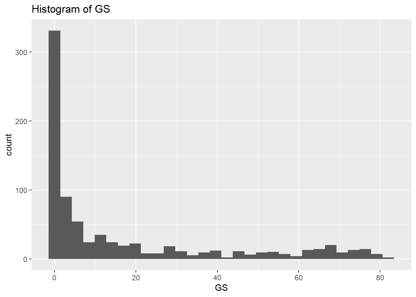
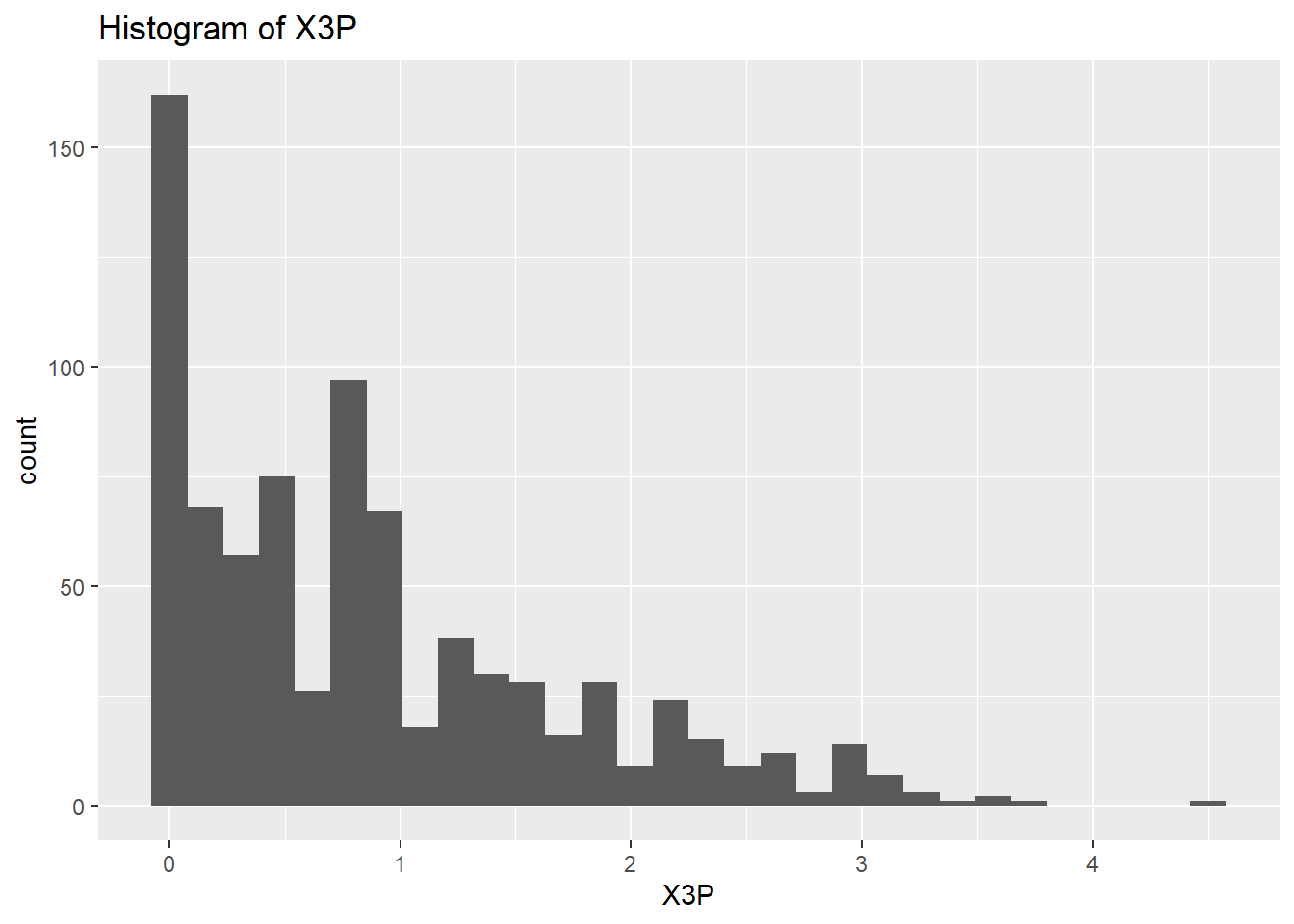
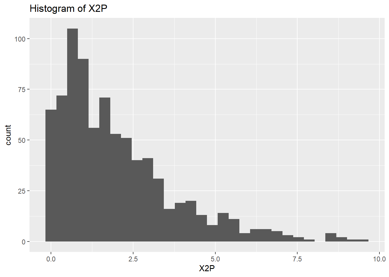
rm(var)So the histograms confirm what we saw from the summary data, we have a long right hand tail for GS but also for X2P and X3P. Let’s check what the boxplots tell us.
# Create a boxplot to check for any outliers
for (var in names(NumericVarsDF)) {
    Box<-ggplot(data = NBADataDF, aes(y = .data[[var]])) +
    geom_boxplot() +
    ggtitle(paste("Boxplot of", var))
  print(Box)
}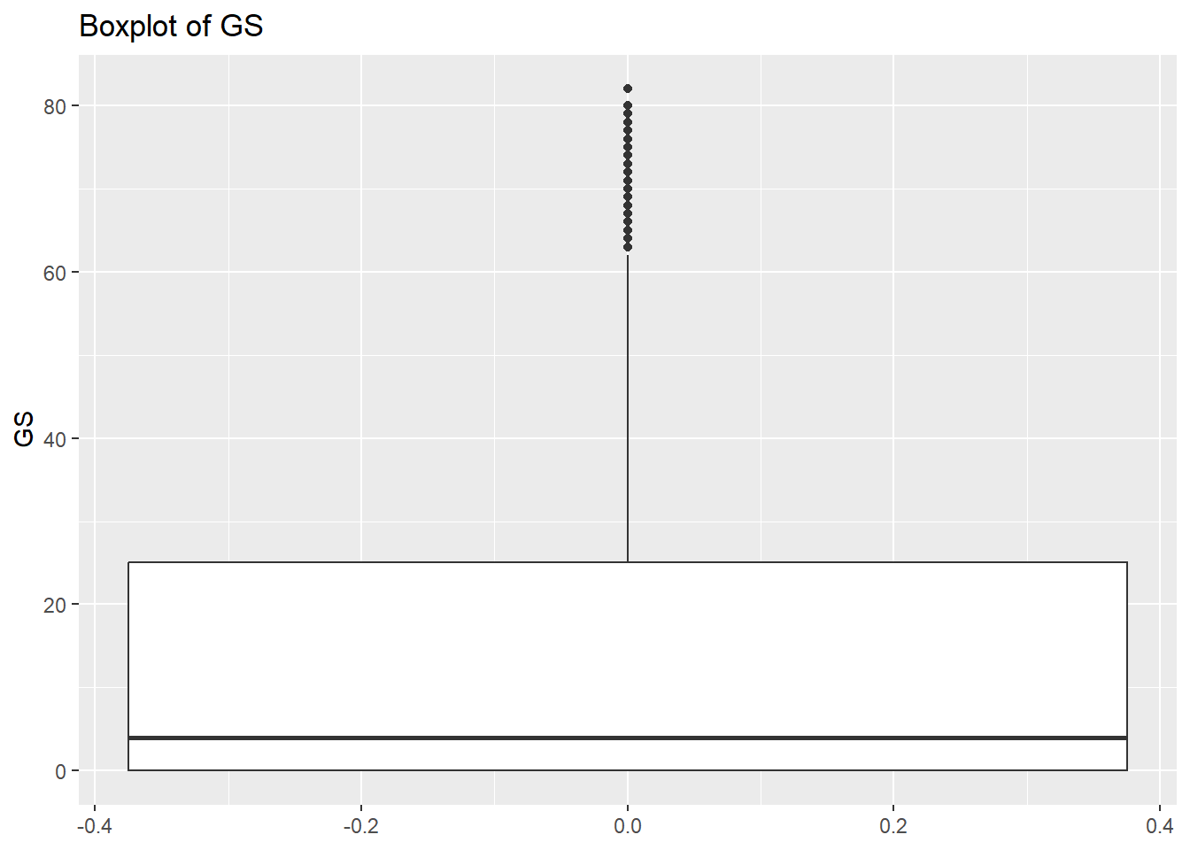
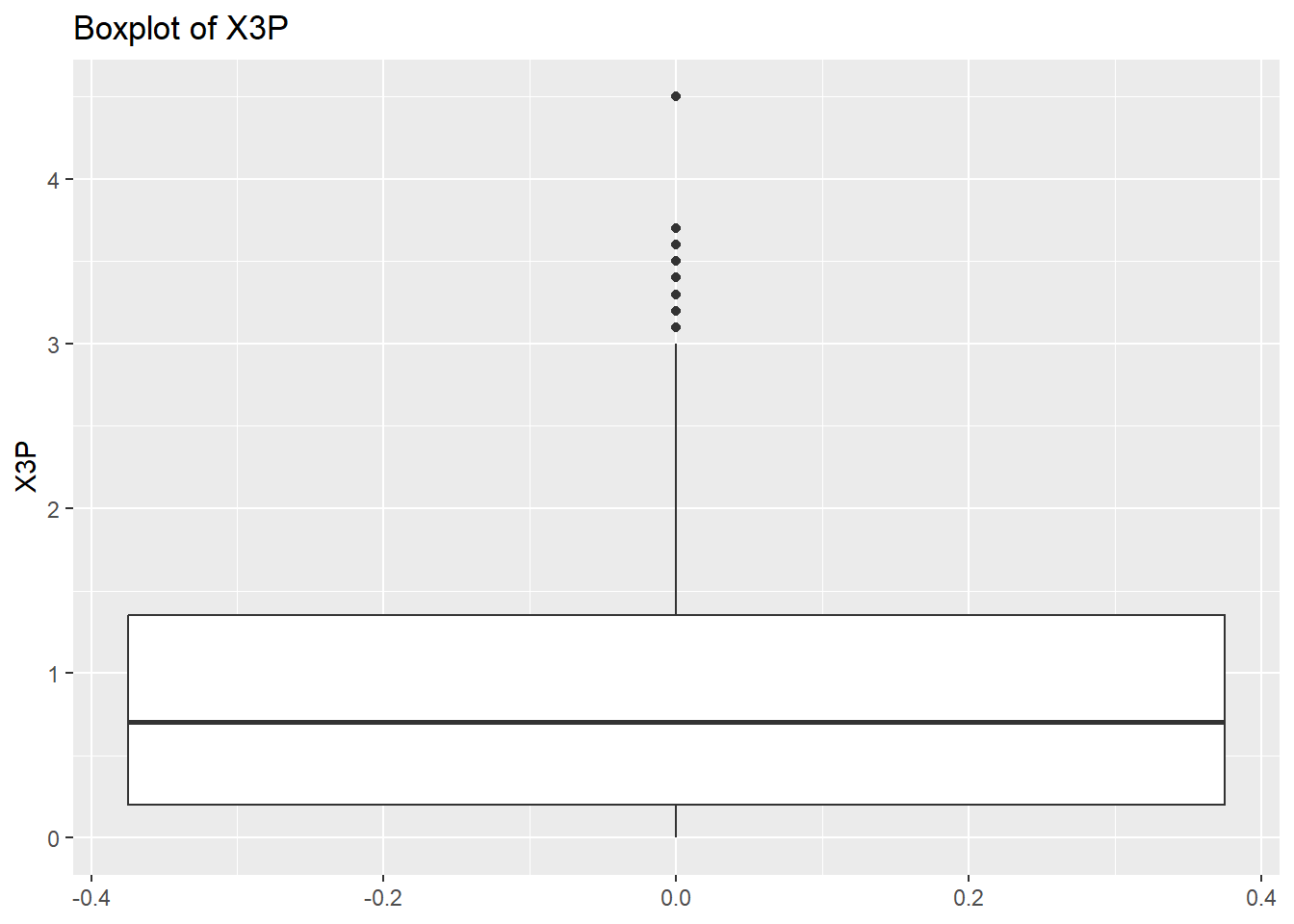
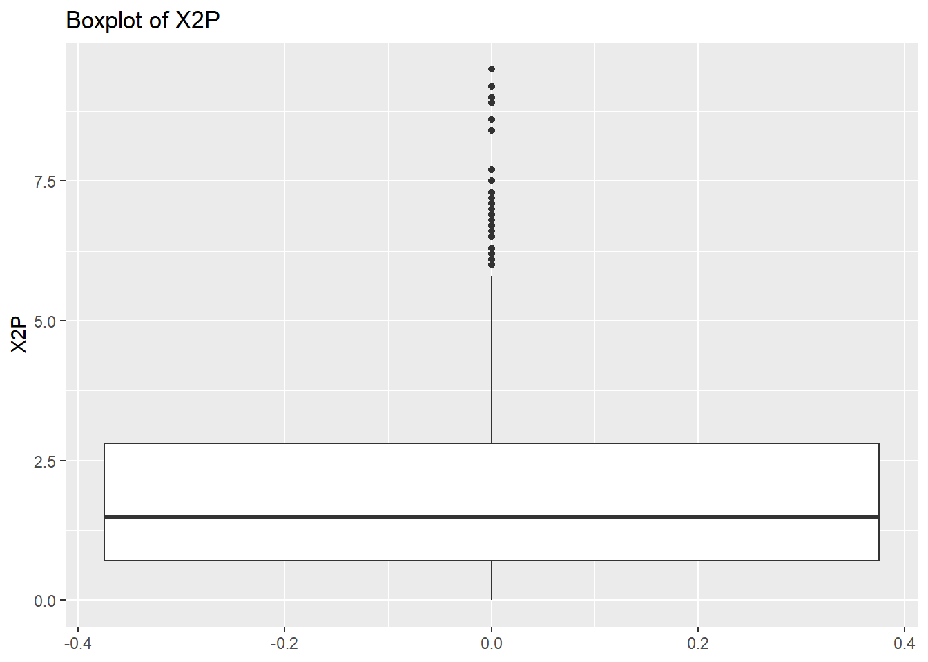
rm(var, NumericVarsDF)Once we have finished cleaning our data we would like to save a clean data set as a .csv file. To do this we can use write.csv() for this.
write.csv(NBADataDF, "C:/Users/wkb14101/OneDrive - University of Strathclyde/MSc SDA/B1701/Practicals/NBADataDF2.csv", row.names=FALSE)Exercise 1: Load the FootballDataP1.csv file located using the following link and on myplace:
Assign your data (as tibble) to FootballDataDF.
FootballDataDF <- as.tibble(read.csv("https://strath-my.sharepoint.com/:x:/g/personal/xanne_janssen_strath_ac_uk/EZ_CnpBOENZCtOLs9EYL0EQBblQliuhwhxkPlVZ8S23Vyw?download=1"))
FootballDataDF
Exercise 2: Check the structure of the FootballDataDF variables and note the different data types. Do you see anything that requires investigating or changing?
# Check NBADataDF
str(FootballDataDF)

# The table below shows several numerical variables (e.g. height, weight) which are categorised as characters. We will need to investigate that. There are also some variables categorised as characters which are grouping variables and should therefore be classed as factors (e.g. preferred_foot or nation_position)
Exercise 3: Create a vector called VariablesToInspect which contains all numerical variables which are currently listed as chr and then create a loop to identify non-numeric values within these variables.
VariablesToInspect <- c("height_cm", "weight_kg")

# Loop through the variables and inspect their unique values
for (var in VariablesToInspect) {
  UniqueValuesDF <- unique(FootballDataDF[grep("[a-zA-Z*-]", FootballDataDF[[var]]), var])
  cat("Unique values in", var, ":\n")
   print(UniqueValuesDF[[var]])
  cat("\n")
}

# The output from the above code shows us that some variables have kg and cm's entered. Before we can assign these variables as numerical we will need to remove these errors.
Exercise 4: Check the gsub() help function to determine what the first three arguments of gsub() need to be. Finish the for loop below in which for each var in VariablesToInspect the “-” gets replaced with ““.
for (….. in ……) {
FootballDataDF[[….]] <- gsub(…, ….., …..)
}for (var in VariablesToInspect) {
FootballDataDF[[var]] <- gsub("[a-z]", "", FootballDataDF[[var]])
}
# The code above has removed the cm and kg text which means we can now change those variables to numeric.Exercise 5: Change the data to numerical using mutate() and across() functions.
FootballDataDF <- FootballDataDF %>%
  mutate(across(c(7,8), as.numeric))
FootballDataDF
Exercise 6: Change preferred_foot, nation_position, team_position, and work_rate from character to factor.
FootballDataDF<- FootballDataDF %>%
  mutate(across(c("preferred_foot", "nation_position", "team_position", "work_rate"), as.factor))
FootballDataDF
Exercise 7: Inspect the column names in the NBADataDF frame.
colnames(FootballDataDF)Exercise 8: Display the columns with missing data.
# Screen for empty variables
cat("Test for empty columns","\n","\n")
EmptyVar <- which(colSums(is.na(FootballDataDF)) == nrow(FootballDataDF))
print(EmptyVar)

# Code shows the defending_marking column is completely empty and we can delete this variable.
Exercise 9: Remove the variables with entirely missing data.
x=0
for (item in EmptyVar) {
  item <- item-x
  FootballDataDF <- FootballDataDF[-item]
  x<- x+1
}
Exercise 10: Check if FootballDataDF has any missing row data and print the total number of missing data points as well as the missing data per variable. Remove any rows which do not have data for the club_name.
cat("Total missing data:","\n", sum(is.na(FootballDataDF)|FootballDataDF==""),"\n")

cat("\n","Missing data per variable:","\n")
print(colSums(is.na(FootballDataDF)|FootballDataDF==""))

FootballDataDF <- FootballDataDF %>%
  filter(club_name!="")
Exercise 11: Scan your data for duplicates using the sofifa_id variable.
# Sort data on player, date and innings number
#| code-fold: true
#| output: false
#| code-summary: "Show the answer"
which(duplicated(FootballDataDF[ ,"sofifa_id"]))integer(0)#No duplicatesExercise 12: Create summary statistics for all numerical variables.
# Check for errors and outliers in each numerical variable
NumericVars <- FootballDataDF %>%
  select_if(is.numeric)
NumericVars <-as.tibble(NumericVars)
NumericVars

# Loop through each numeric variable

for (var in names(NumericVars)) {
  # Calculate summary statistics
  VarSummary <- summary(NumericVars[[var]],na.rm=TRUE)

  # Print summary statistics and outliers
  cat("Variable:", var, "\n")
  print(VarSummary)
  cat("\n")
  }
Exercise 13: Create histograms and boxplots for height_cm, weight_kg, and value_eur
# Create a histogram to visualize the distribution and check for any outliers
NumericVars <- select(FootballDataDF, c("height_cm", "weight_kg", "value_eur"))

for (var in names(NumericVars)) {
    histo<-ggplot(data = FootballDataDF, aes(x=.data[[var]])) +
    geom_histogram() +
    ggtitle(paste("Histogram of", var))
  print(histo)
}# Create a boxplot to check for any outliers
for (var in names(NumericVars)) {
Box<-ggplot(data = FootballDataDF, aes(y = .data[[var]])) +
geom_boxplot() +
ggtitle(paste("Boxplot of", var))
print(Box)
}Exercise 14: Looking at the boxplots, what can you say about them?
# Height and weight are fairly normally distributed with a few outliers at the top and bottom ranges. Players value shows some very extreme outliers with the distribution heavily skewed to the right (creating an inflated mean).Exercise 15: Save your data.
write.csv(FootballDataDF, "C:/Users/wkb14101/OneDrive - University of Strathclyde/MSc SDA/B1701/Practicals/FootballDataDF.csv", row.names=FALSE)